
saving more with mixed-integer programming
Published:
As a rite of passage for every new homeowner, my wife and I recently went down the rabbit hole of trying to find the best deal for the major appliances in our new home. That was when we came across an Audio House appliance promotion that combined invoice discounts, cashback, and enough terms and conditions to make manual calculation unreliable:
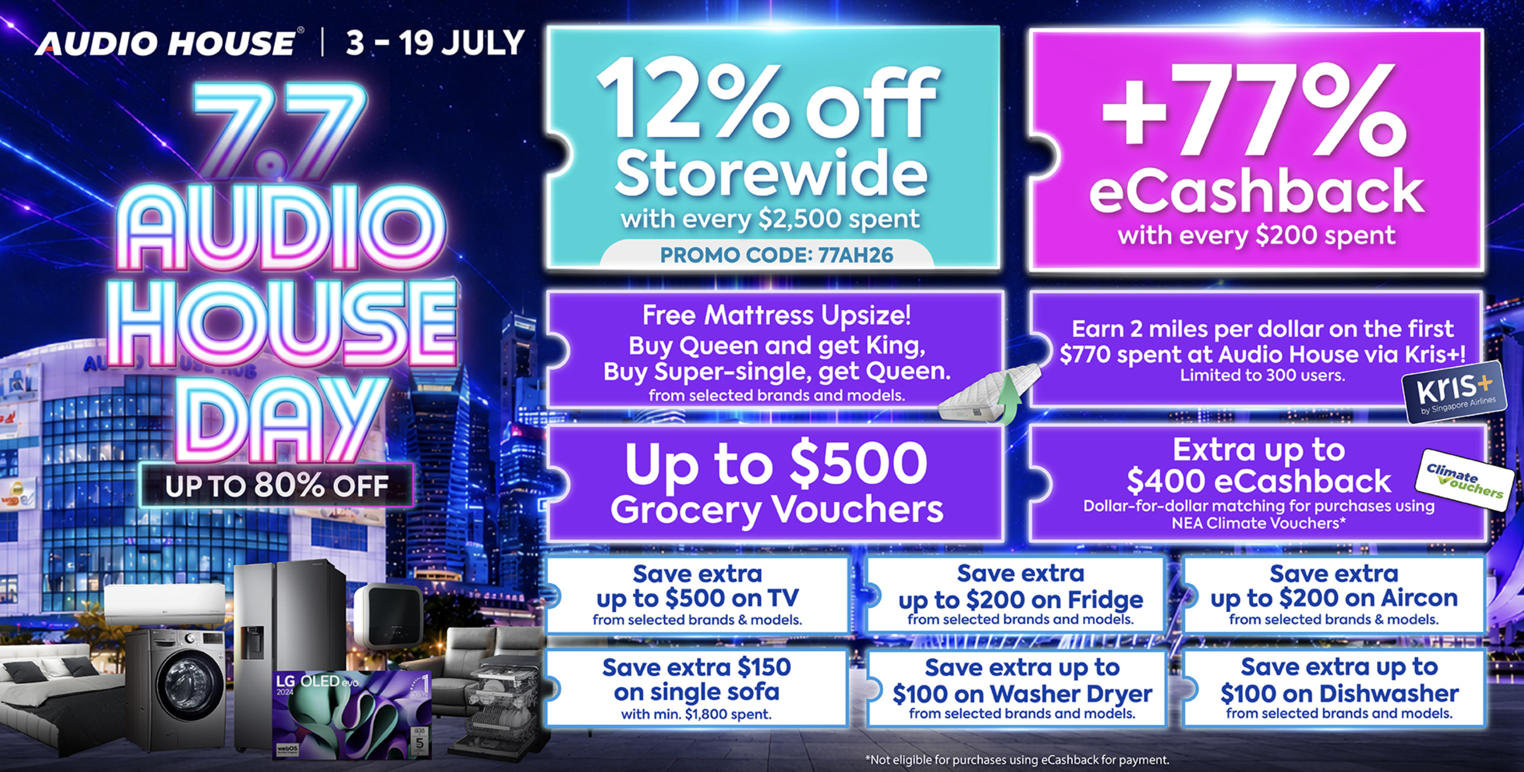
An impressive amount of fine print for a single shopping trip.
At first glance, it was hard to tell whether this was a great deal or an elaborate trap for tired homeowners. The core mechanic of the cashback promotion, however, was simple enough:
- Buy some items in the first invoice.
- Earn cashback from that invoice.
- Use that cashback immediately on the second invoice, subject to a redemption cap.
That sounds manageable until the terms and conditions show up. The promotion was not just “spend more, save more.” It had several interacting rules:
- Every complete
$2,500of discount-eligible spend gives a$300invoice discount. - The discount is calculated independently on each invoice.
- Every complete
$200of cashback-eligible spend on Invoice 1 gives$154of cashback. - Earned cashback is rounded down to the nearest
$20. - Cashback redemption on Invoice 2 is capped at 20% of Invoice 2 after discounts, also rounded down to the nearest
$20. - Some items are eligible for discount, some for cashback, some for both, and some for neither.
- A multi-quantity item can be split across the two invoices.
- Existing cashback can be added on top of newly earned cashback, but it still cannot exceed the Invoice 2 cap.
Soon it became clear that this was no longer something we wanted to settle with rough spreadsheet math. Apparently the salespeople would help do the arithmetic on the spot, but that mostly meant scribbling on paper or tapping numbers into a phone calculator. We wanted a more defensible way to optimize the invoice split and total savings.
How do we calculate the best deal?
This is a small resource-allocation problem, which makes it a nice fit for combinatorial optimization. More specifically, I modelled the appliance cashback problem as a mixed-integer linear program, a close cousin of the knapsack problem.
The goal was to split the shopping cart into two invoices:
- Invoice 1 should earn as much useful cashback as possible.
- Invoice 2 should be large enough, and structured well enough, to redeem that cashback.
- Both invoices should also collect as many
$2,500 -> $300discount blocks as possible.
That “useful” part matters. Maximizing cashback earned is not the same as maximizing total savings, because cashback is only valuable if Invoice 2 is able to redeem it. A naive strategy can earn a lot on the first invoice and then get blocked by the redemption cap on the second.
I turned that into a small Python app called audiohouse, backed by FastAPI and a PuLP mixed-integer model. The app works as an invoice split optimizer: it decides how many units of each item should go into Invoice 1, with the remaining units automatically going into Invoice 2.
I had only seen this kind of optimization in coursework and toy exercises before. The fun part here was translating a real sales promotion into equations without accidentally simplifying away the annoying details that actually change the answer.
Turning the promotion rules into equations
Suppose item i has:
- unit price
P_i - quantity
Q_i - cashback flag
E_i, which is 1 if the item is cashback-eligible - discount flag
V_i, which is 1 if the item is discount-eligible
The key decision is:
\[x_i = \text{number of units of item } i \text{ assigned to Invoice 1}\]with
\[0 \le x_i \le Q_i\]and the remaining quantity
\[Q_i - x_i\]going to Invoice 2.
This is already enough to encode one of the practical quirks of the promotion: if an item has quantity greater than 1, the solver is allowed to split it across invoices instead of forcing the whole line item onto one side.
1. Volume discount
For discount purposes, only discount-eligible spend counts toward the $2,500 threshold.
Each complete $2,500 block gives a $300 discount, so if d_1 and d_2 are the number of complete discount blocks:
subject to
\[2500 d_1 \le T_1^{disc},\qquad 2500 d_2 \le T_2^{disc}\]This captures the “floor” behavior without writing floor functions directly into the optimizer.
One subtle detail from the actual promotion is that a non-discount-eligible item can still be useful. It does not help create a $2,500 block, but it may still belong on a particular invoice because of cashback or because it helps shape the second invoice’s redemption cap.
2. Cashback earned on Invoice 1
Only cashback-eligible spend on Invoice 1 contributes to earned cashback:
\[T_1^{cash} = \sum_i E_i P_i x_i\]Every complete $200 gives $154 of raw cashback. If b_1 is the number of complete $200 blocks, then:
with
\[200 b_1 \le T_1^{cash}\]The promotion then rounds earned cashback down to the nearest $20. In the implementation, that is represented with another integer helper variable so that:
and
\[20 c_{earned} \le 154 b_1\]This means a single $200 block does not produce usable cashback of $154; it produces $140 after rounding.
3. Cashback redeemed on Invoice 2
Invoice 2 may redeem cashback, but only up to 20% of its post-discount total. First define the gross second invoice:
\[T_2 = \sum_i P_i (Q_i - x_i)\]Then the redemption cap is:
\[C_{cap} = 20 c_{max}\]with
\[20 c_{max} \le 0.2 (T_2 - D_2)\]Again, the $20 granularity is deliberate: even the cap is rounded down.
If there is already some cashback sitting around from a previous purchase, call it C_{extra}. The total redeemable cashback is then bounded by both the available cashback and the cap:
That second constraint is why maximizing earned cashback alone can fail. A large Invoice 1 is only half the story; Invoice 2 must still be able to absorb the cashback.
4. Objective
The optimization target is the total savings:
\[S = D_1 + D_2 + C_{redeemed}\]So the solver simply maximizes S.
That sounds obvious, but it is the difference between a correct optimization model and a misleading heuristic. The best split would have to be the one that balances all three savings components rather than pushing one of them to the extreme.
A small invoice split example
Here is the kind of tradeoff the solver handles well.
Suppose we want to buy:
| Item | Price | Qty | Cashback eligible? | Discount eligible? |
|---|---|---|---|---|
| Washer | $1,200 | 1 | Yes | Yes |
| Dryer | $1,100 | 1 | Yes | Yes |
| Fridge | $2,600 | 1 | No | Yes |
| Hood | $500 | 1 | Yes | No |
I might have instinctively put the two cashback-eligible appliances on Invoice 1 to maximize earned cashback. But that can be suboptimal if Invoice 2 becomes too small to redeem much of it.
The solver instead evaluates all valid integer splits and may choose something less obvious, such as pushing more discount-eligible value into Invoice 2 so that:
- Invoice 1 still crosses enough
$200cashback blocks to matter. - Invoice 2 keeps a large enough post-discount total to raise the 20% redemption cap.
- Both invoices have a chance to hit a
$2,500discount block.
This is exactly the kind of situation where “calculator math” starts to break down. Each local improvement can make another part of the promotion worse. It is also why an optimization model is more reliable than trying to estimate the best cashback split by inspection. But that being said, the salesperson that engaged us at the actual store did all of this with just a sheet of paper, a calculator, and 20 minutes of number crunching :)
So…
The project itself is small, but I chose to write about it because the constraints are concrete. There is no abstract warehouse, no fictional truck loading problem, and no sanitized textbook phrasing. Just a new homeowner trying his luck at better savings (with enough edge cases to force a proper model!)
It also reminded me that many real optimization problems are not hard because the math is exotic. They are hard because the rules are messy, the rounding is annoying, and the obvious strategy is only locally sensible.
If you want to see the implementation, the repository is here: jylee-k/audiohouse. It exposes the solver through a small FastAPI endpoint and a simple browser UI, but the interesting part is really the mixed-integer programming model in solver.py.
Dedicating this post to my wife who inspired this little project :)